
Discovering Interpretable Omic Networks with gPCR.
Standard SVAES can predict outcome, but not the true network behind it. A new method called gPCR does both, and could transform how scientists design experiments.

Uncovering Predictive Networks, an Impossible Goal?
Imagine you spend months running experiments to identify which proteins in the brain drive Alzheimer’s disease progression. You build a model, it predicts outcomes beautifully, and you use it to pick targets for intervention. Then the intervention fails, not because the biology was wrong, but because the model’s predictions and its internal network representation were quietly disagreeing with each other the whole time. This is not a hypothetical. It is a structural flaw in one of the most widely used classes of machine learning models in science today. A new paper from researchers at Emory, Stanford, Duke, and UC Davis introduces a method called generative principal component regression (gPCR) that addresses this flaw head-on.
The problem: two goals, one model
Scientists working with high-dimensional data, thousands of proteins, hundreds of neural frequency bands, tens of thousands of gene expression measurements, face a fundamental tension. On one hand, they want interpretability. Factor models like PCA compress data into a small number of latent “networks,” each corresponding to some underlying biological process. These networks are scientifically meaningful: they can be measured, targeted, and manipulated. On the other hand, they want predictive accuracy. When trying to predict whether a patient has Alzheimer’s, or whether a mouse is under stress, pure interpretability is not enough, you need a model that actually gets the right answer. The standard approach to combining these is principal component regression (PCR): first run PCA to find the latent networks, then regress the outcome on those networks. The problem is that PCA finds the directions of maximum variance in the data, not the directions most predictive of the outcome. If the biologically relevant signal happens to be low-variance, which it often is, PCR misses it entirely.
Supervised Variational Autoencoders: A silver bullet?
Supervised variational autoencoders (SVAEs) try to solve this by adding a predictive objective on top of the generative model. The idea is appealing: train the model to both reconstruct the data and predict the outcome, and you should get representations that are both interpretable and predictive. But SVAEs have a critical structural problem. They use two separate components to do their work: an encoder (which maps observations to the latent space) and a decoder (which reconstructs observations from the latent space). The supervision loss acts only on the encoder, so the encoder learns to represent the outcome well, but the decoder, which defines the generative model and its scientifically interpretable loadings, does not. In other words, the encoder and decoder end up describing two different latent spaces. The encoder says “this brain state is associated with stress.” The decoder says something different. When you use the decoder’s loadings to design a stimulation experiment — as neuroscientists actually do — you are acting on a representation that does not match the model’s own predictions.
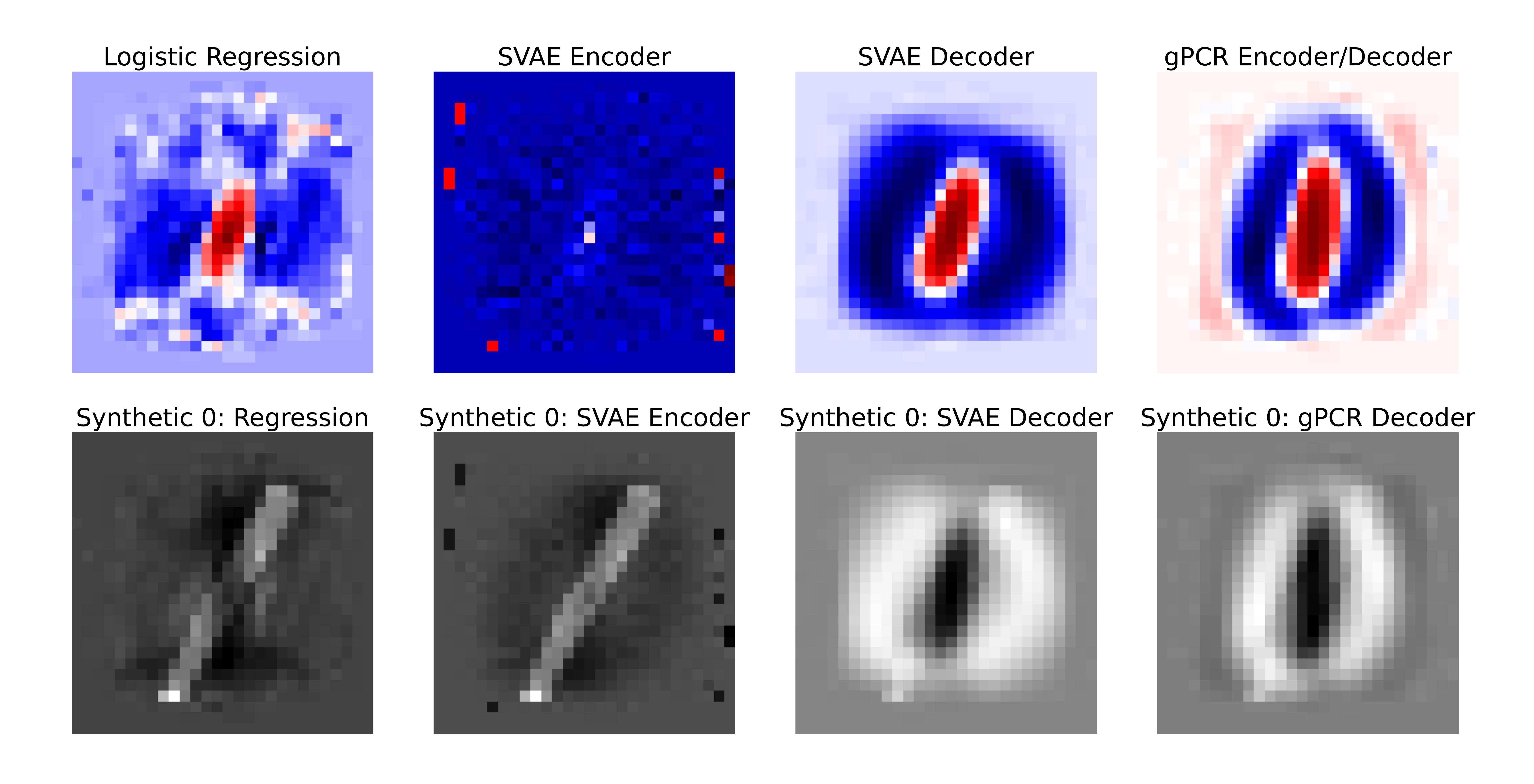
We demonstrate this vividly with MNIST digits. They train all three models (logistic regression, SVAE, and gPCR) to distinguish 0s from 1s, then ask each model to “convert” a 1 into a 0 by shifting the image in the direction the model says matters. The SVAE encoder produces a manipulation that its own decoder says is still a 1. gPCR produces a clean, recognizable 0.
The gPCR solution
The key insight behind gPCR is simple: instead of using a flexible encoder that can drift away from the generative model, constrain the encoder to always equal the generative posterior. This means the latent space the model uses for prediction is the same latent space defined by the generative model’s loadings. Mathematically, gPCR maximizes a weighted objective: the standard generative log-likelihood plus a predictive term, where the expectation in the predictive term is taken under the generative posterior rather than a separate encoder distribution. This forces any predictive information to be reflected in the loadings themselves. For linear Gaussian models the generative posterior has a closed form, making this tractable and computationally efficient. The per-iteration cost matches that of standard penalized regression. There is also a supervision strength parameter, but unlike in standard regression, gPCR is relatively insensitive to its precise value. Below a critical threshold, the model behaves like PCA. Above it, it locks on to the predictive subspace. The plateau of good performance is wide, which makes tuning straightforward.
Results: neuroscience and Alzheimer’s
The authors validate gPCR on three real datasets.
Electrophysiology: predicting brain region activity. Using recordings from mice in a stress task, gPCR dramatically outperformed standard PCR and matched the performance of Elastic Net regression — a dedicated predictive model — while retaining the network interpretation PCR provides.
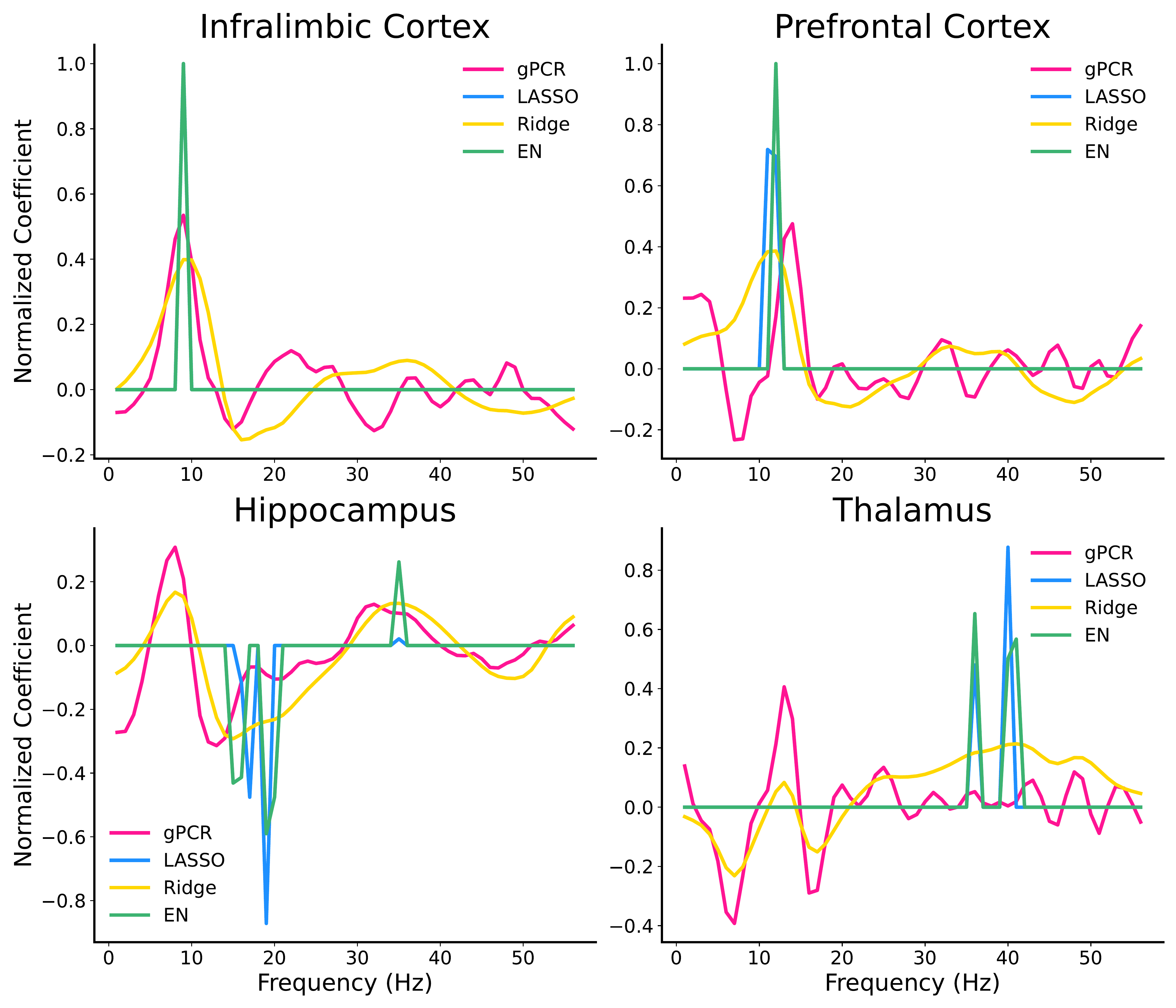
Electrophysiology: predicting social behavior. In a harder task (distinguishing social from non-social interaction), gPCR outperformed LASSO regression and matched Ridge and Elastic Net, despite also having to reconstruct the data. Perhaps more importantly, the coefficients it learned aligned with natural neural frequency bands — unlike LASSO, which arbitrarily zeroed out neighboring frequencies.
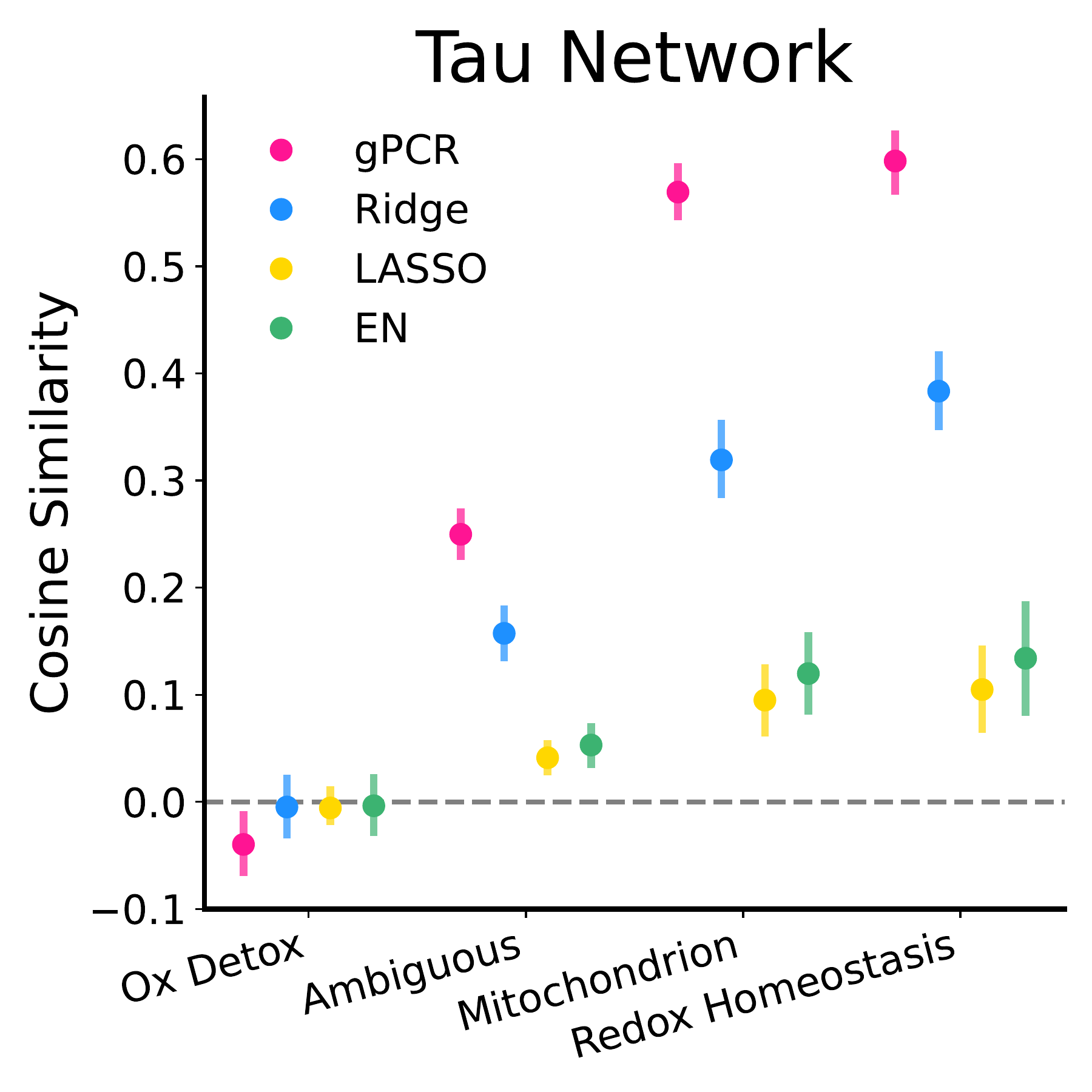
Proteomics: Alzheimer’s phenotypes. On a cohort of 300 individuals (140 healthy controls, 160 with Alzheimer’s), gPCR predicted tau tangle and beta amyloid levels as well as the best regression methods, while standard PCR failed. More strikingly, the networks gPCR identified, such as redox homeostasis, oxidant detoxification, mitochondrial function, ubiquitination, align closely with established Alzheimer’s biology. The regression methods did not show the same alignment.
Why this matters for experimental design
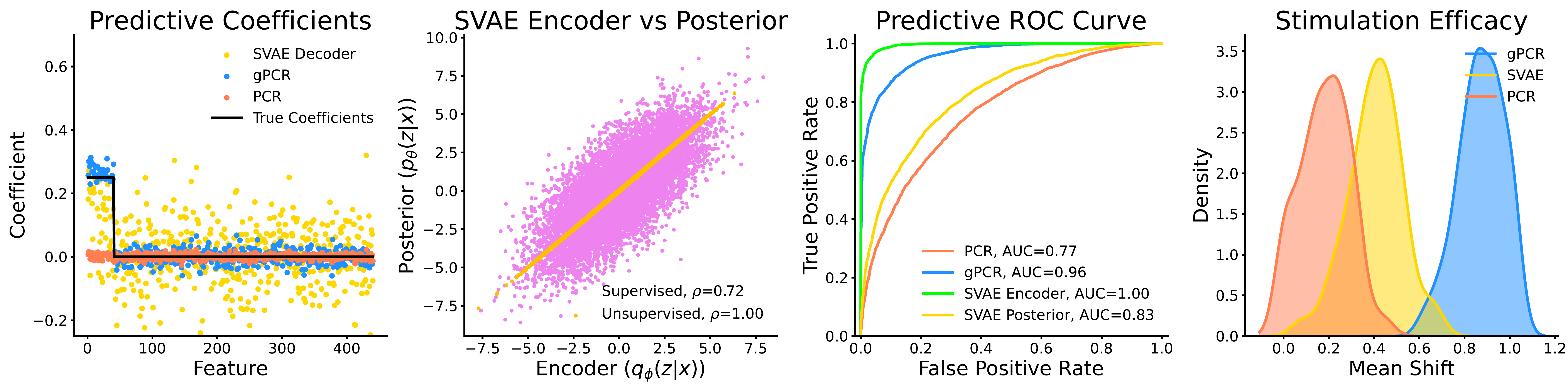
The practical stakes here are high. In neuroscience, stimulation experiments are designed based on model loadings: you identify which features (frequency bands, brain regions) are most associated with a latent factor, then apply a targeted stimulus to those features. If the model’s loadings do not actually represent the predictive subspace, which we show is the case for SVAEs, then the stimulation protocol is fundamentally skewed. In the synthetic experiments, gPCR-based stimulation protocols produced an average phenotype shift of 0.89, compared to 0.41 for SVAE and 0.18 for PCR. In a real experiment, that difference could be the gap between a successful intervention and a null result.
Limitations and what comes next
gPCR currently requires the generative posterior to have a closed form, which restricts it to linear Gaussian models. This covers a wide range of applications, but nonlinear relationships between latent variables and observations are left for future work. The authors suggest MCMC-based sampling from the posterior as a potential path forward, at the cost of increased computational complexity. The method also depends on covariance estimation, which can become unstable under extreme data sparsity. This is a common limitation of any second-order statistical approach. Code is available in the Bystro GitHub repository.
The bottom line
gPCR is a principled solution to a problem that has quietly undermined scientific inference in latent variable modeling for years. It matches the predictive performance of regression while preserving the network interpretation of generative models, and unlike SVAEs, it ensures those two things are actually consistent with each other. For researchers who use their models not just to predict but to understand and intervene, that consistency is not a nice-to-have. It is the whole point.
Written by Austin Talbot, Head of ML at bystro.
Read the full publication: